Query Optimization and Equivalence
Query Optimization Example
A single query can be executed in multiple ways depending on the order of operations. The database optimizer analyzes these options to choose the most efficient path.
Consider a database with these schemas:
course (course_id, title, dept_name, credits)
instructor (ID, name, dept_name, salary)
teaches (ID, course_id, sec_id, semester, year)
Goal: Select the course instructor name and title who belongs to the department ‘Music’.
Here are two possible evaluation plans for the exact same query:
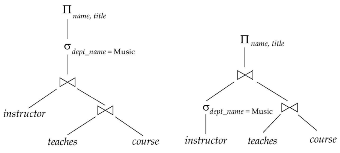
The optimizer will calculate the cost of both plans and choose the one that executes faster (typically the one that reduces the dataset size earlier by performing the Selection operation before the Join).
Equivalence Rules
How does the database optimizer know that two different execution plans will return the exact same result? It relies on Equivalence Rules.
These mathematical rules state that certain relational algebra expressions can be transformed into other expressions without changing the final output. The optimizer applies these rules to rewrite the query into a more efficient form.
1. Selection Rules
Conjunctive selections can be split: A selection with multiple conditions connected by AND (\(\land\)) can be broken down into a sequence of individual selections. \[ \sigma_{\theta_1 \land \theta_2}(E) = \sigma_{\theta_1}(\sigma_{\theta_2}(E)) \]
Selections are commutative: The order in which you apply filters doesn’t matter. \[ \sigma_{\theta_1}(\sigma_{\theta_2}(E)) = \sigma_{\theta_2}(\sigma_{\theta_1}(E)) \]
2. Projection Rules
- Only the final projection matters: In a sequence of projection operations, only the last one is necessary; the others can be safely omitted. \[ \Pi_{L_1}(\Pi_{L_2}(...\Pi_{L_n}(E)))) = \Pi_{L_1}(E) \]
3. Join Rules
Theta-joins are commutative: Joining Table A to Table B gives the same result as joining Table B to Table A. \[ E_1 \bowtie_\theta E_2 = E_2 \bowtie_\theta E_1 \]
Natural joins are associative: When joining three tables, it doesn’t matter which two you join first. \[ (E_1 \bowtie E_2) \bowtie E_3 = E_1 \bowtie (E_2 \bowtie E_3) \]
Selections can be combined with Cartesian products to form a join: \[ \sigma_{\theta}(E1 \times E2) = E_1 \bowtie_\theta E_2 \]
Selections can be absorbed into a join condition: \[ \sigma_{\theta_1}(E_1 \bowtie_{\theta_2} E_2) = E_1 \bowtie_{\theta_1 \land \theta_2 } E_2 \]
4. Set Operation Rules
- Associative:
- Union: \((E_1 \cup E_2) \cup E_3 = E_1 \cup (E_2 \cup E_3)\)
- Intersection: \((E_1 \cap E_2) \cap E_3 = E_1 \cap (E_2 \cap E_3)\)
- Commutative:
- Union: \(E_1 \cup E_2 = E_2 \cup E_1\)
- Intersection: \(E_1 \cap E_2 = E_2 \cap E_1\)
- (Note: Set difference is NOT commutative)
- Projection distributes over union: \[ \Pi_L(E_1 \cup E_2) = (\Pi_L(E_1)) \cup (\Pi_L(E_2)) \]