Hashing and Bitmap Indices
What is Hashing?
Instead of searching through a sorted structure, hashing computes exactly which bucket a record lives in — no traversal needed. Think of it as a direct address calculator.
A hash function \(h\) maps a search key to a bucket address:
\[h : \text{search-key values} \rightarrow \text{bucket addresses}\]
- A bucket is a unit of storage — typically one disk block — holding one or more records.
- If \(h(k_1) = h(k_2)\) for \(k_1 \neq k_2\), a collision has occurred.
A good hash function is uniform (distributes keys evenly across all buckets) and fast to compute.
⚠️ The worst hash function maps every key to the same bucket — search degrades to \(O(n)\).
Static Hashing
The number of buckets \(B\) is fixed at creation time.
Lookup: compute \(h(k)\) → go directly to that bucket → scan within it sequentially.
Example: 10 buckets, keys are department names. Hash = sum of character values mod 10.
h(Music)      = 1    h(History)   = 2
h(Physics)    = 3    h(Elec. Eng.) = 3   ← collision
Physics and Elec. Eng. both map to bucket 3. Both records are stored there and the bucket is scanned sequentially to find the right one.
Handling Bucket Overflow
Overflow happens when a bucket fills up. Causes:
- Too few buckets allocated initially.
- Skew — many records share the same key, or the hash function distributes unevenly.
Solution: overflow chaining — link overflow buckets to the original in a linked list.
Bucket 3: [Physics | Elec. Eng.] → [overflow block] → ...This scheme is called closed hashing.
Deficiencies of Static Hashing
The fixed bucket count \(B\) is the core problem:
| Scenario | Problem |
|---|---|
| File grows beyond initial estimate | Too many overflow chains → poor performance |
| File shrinks | Mostly empty buckets → wasted space |
| \(B\) set too large from the start | Space wasted immediately |
Periodic full reorganization with a new hash function is possible but expensive and disruptive.
Better fix: let the number of buckets grow and shrink dynamically.
Dynamic Hashing (Extendable Hashing)
Instead of a fixed bucket count, extendable hashing uses a directory (bucket address table) that doubles or halves as needed.
Core Idea
- The hash function produces a \(b\)-bit integer (typically \(b = 32\)).
- Only the first \(i\) bits (global depth) are used to index into the directory.
- Directory size = \(2^i\). Initially \(i = 0\).
- Each bucket \(j\) stores its own local depth \(i_j\) — how many bits actually identify its entries.
- Multiple directory entries can point to the same bucket when \(i_j < i\).
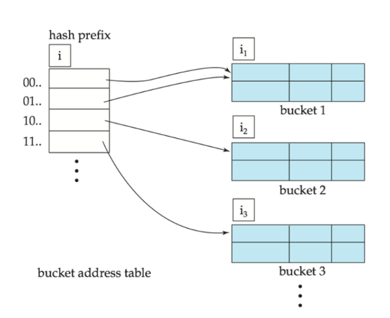
Lookup
- Compute \(h(k) = X\).
- Use the first \(i\) bits of \(X\) as a directory index.
- Follow the pointer to the bucket and scan within it.
Insertion
- Lookup the target bucket \(j\).
- If space exists → insert. Done.
- If bucket \(j\) is full → split:
Case 1 — \(i > i_j\) (multiple entries point to \(j\)): - Allocate new bucket \(z\), set \(i_j = i_z = i_j + 1\). - Redirect the second half of entries that pointed to \(j\) → now point to \(z\). - Redistribute all records in \(j\) between \(j\) and \(z\) by recomputing hash prefixes. - Retry insertion.
Case 2 — \(i = i_j\) (only one entry points to \(j\)): - Increment \(i\), double the directory (each old entry becomes two entries pointing to the same bucket). - Now \(i > i_j\) → apply Case 1. - If \(i\) hits limit \(b\) or too many splits occur, use an overflow bucket instead.
Deletion
- Remove the record from its bucket.
- If the bucket empties, it can be removed.
- Coalesce with a “buddy” bucket — a bucket with the same \(i_j\) and the same \((i_j - 1)\)-bit prefix.
- Shrink the directory if the actual bucket count becomes much smaller than \(2^i\) (expensive — do sparingly).
Extendable Hashing: Pros and Cons
| ✓ Advantages | ✗ Disadvantages |
|---|---|
| Performance doesn’t degrade as file grows | Extra level of indirection on every lookup |
| Minimal space overhead | Directory can exceed memory size |
| No periodic reorganization needed | Doubling the directory is expensive |
💡 If the directory outgrows memory, a B+ tree can index into it — combining the benefits of both structures.
Bitmap Indices
Bitmap indices are designed for multi-attribute analytical queries on low-cardinality columns — not for point lookups.
What They Are
For an attribute with \(m\) distinct values, a bitmap index stores \(m\) bit vectors — one per distinct value. Each bit vector has one bit per record:
- 1 if the record has that value.
- 0 otherwise.
Example: gender attribute, 5 records:
Record:     0  1  2  3  4
Gender:     M  F  M  F  M

Bitmap(M):  1  0  1  0  1
Bitmap(F):  0  1  0  1  0
📌 Best suited for columns with few distinct values — gender, country, income bracket, status flags. Not useful for high-cardinality columns like names or IDs.
Answering Queries with Bitmaps
Multi-attribute queries use bitwise operations — extremely fast at the CPU level.
| Operation | Meaning |
|---|---|
| AND | Records matching both conditions |
| OR | Records matching either condition |
| NOT | Records not matching a condition |
Example: find male instructors at income level L1:
Bitmap(gender=M):    1 0 0 1 0
Bitmap(income=L1):   1 0 1 1 0
                     ---------
AND result:          1 0 0 1 0   → records 0 and 3 match