Relational Model & DDL

What is a Relational Database?

Before diving into commands, let’s build some intuition. Imagine a school register. You have a list of students, their roll numbers, and the courses they are taking. In a Relational Database, we store data in structured tables (also called relations). Every row represents a single entity (like one specific student), and every column represents an attribute of that entity (like their name or grade).

The true power of relational databases isn’t just storing tables—it’s how we can relate them using Keys, and slice them using mathematical operations!

The Concept of Keys

In a database, we need a way to uniquely identify every row so we don’t confuse two students named “John Smith”. We do this using Keys.

Super Key: Any combination of columns that can uniquely identify a row. For a student, [Roll Number, Name] is a super key, but it’s bulkier than it needs to be.
Candidate Key: A minimal Super Key. It has no unnecessary columns. Both [Roll Number] and [Email Address] could be candidate keys.
Primary Key: The one Candidate Key you officially choose to identify your rows. Once chosen, no two rows can have the same Primary Key, and it cannot be empty.
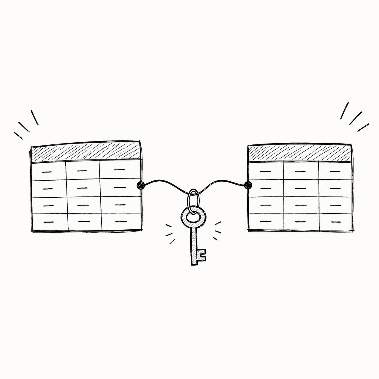
Surrogate Key: Sometimes, natural data (like names) makes for bad keys. A Surrogate Key is an artificially generated ID (like an auto-incrementing Student_ID = 1, 2, 3...) created purely to act as the Primary Key.
Foreign Key: This is the literal glue that makes a database “relational”! A Foreign Key is a column in Table A that points exactly to the Primary Key in Table B. It links the two tables together.

Example: The student_id column in the Grades table is a Foreign Key that points to the student_id Primary Key in the Student table.

Relational Queries & The Pure Language

How do we ask a database for information? We use a Query Language.

There’s a fundamental difference in how these languages work:

Imperative Languages (like Python or Java): You must write step-by-step instructions on how to find the data.
Declarative Languages: You simply describe what data you want, and the system figures out the best way to get it.

Before modern SQL existed, computer scientists created “pure” theoretical languages to prove databases could work. Relational Algebra is one of these pure languages. It uses mathematical symbols to describe exactly how to slice and dice tables.

Relational Operators: Slicing and Dicing

Relational Algebra gives us Relational Operators—surgical tools to extract what we need.

The Big Two: Select vs. Project

Select (\(\sigma\)): Filters Rows. It scans horizontally. (e.g., “Find all students who got an ‘A’”).
Project (\(\pi\)): Filters Columns. It scans vertically. (e.g., “I only need to see Names and Roll Numbers”).

%%{init: {'theme': 'neutral'}}%%
graph LR
    classDef default fill:#ffffff,stroke:#333,stroke-width:2px,color:#000000;
    classDef sub fill:#f0f0f0,stroke:#666,stroke-width:2px,color:#000000;

    subgraph original[Original Table]
        A["Row 1, Col X, Col Y"]
        B["Row 2, Col X, Col Y"]
        C["Row 3, Col X, Col Y"]
    end

    subgraph select_op[Select Operation]
        S1["Row 1, Col X, Col Y"]
        desc1["(Filters Rows)"]
    end
    
    subgraph project_op[Project Operation]
        P1["Col X only"]
        desc2["(Filters Columns)"]
    end

    original -- Select --> select_op
    original -- Project --> project_op

Other Important Operators

Operator	Symbol	Intuition	Everyday Example
Union	\(\cup\)	Combines two sets into one big list.	“Give me the list of students in the morning class PLUS the evening class.”
Intersection	\(\cap\)	Returns items present in both sets.	“Who is taking BOTH Physics AND Chemistry?”
Set Difference	\(-\)	Returns items in the first set but NOT in the second.	“Students taking Physics but NOT taking Chemistry.”
Cartesian Product	\(\times\)	Combines every row of one table with every row of another.	Matching every color of a shirt with every size available.
Natural Join	\(\bowtie\)	Connects two tables seamlessly based on matching columns.	Linking the `Student` table to the `Grades` table.

What is SQL?

While Relational Algebra is great for theory, we needed a real, practical language to type into a computer. Enter SQL (Structured Query Language).

A Brief History: Developed at IBM in the 1970s by Donald Chamberlin and Raymond Boyce, SQL was initially called “SEQUEL”. It was designed to manipulate data stored in IBM’s quasi-relational database management system. Over the decades, it became the undisputed, standardized language for relational databases globally.

SQL is broadly divided into three main categories:

DDL (Data Definition Language): Used to define the structure (the blueprint).
DML (Data Manipulation Language): Used to insert, update, and query the actual data (the furniture).
DCL (Data Control Language): Used to manage permissions and security (the bouncers).

Domain Types & Integrity Constraints

Before building our table, we must set the rules.

Domain Types

We must tell the system what kind of data a column stores. This prevents someone from typing “Twenty” into an Age column.

Type	Description	Example
`char(n)`	Fixed-length text. Good for Zip Codes.	`char(5)` pads “Hi” to `"Hi "`
`varchar(n)`	Variable-length text. Good for names.	`varchar(50)` stores “Hi” as `"Hi"`
`int`	A whole number.	`25`
`numeric(p,d)`	A decimal number. `p` is total digits, `d` is after the decimal.	`numeric(4,2)` allows `44.22` but rejects `100.22`

Integrity Constraints

Constraints are extra rules we apply to columns to ensure the data makes sense.

NOT NULL: The column cannot be left empty.
UNIQUE: No two rows can have the same value in this column.
CHECK(condition): Ensures the value meets a specific requirement (e.g., CHECK (age >= 18)).
PRIMARY KEY: Automatically enforces both UNIQUE and NOT NULL.

DDL: Building the Blueprint

Intuition: DDL is the architect. You use DDL to draw the blueprints and set the rules. DDL does not handle the actual data.

1. The `CREATE` Command

We use CREATE TABLE to bring a new table into existence. Let’s create a student table with constraints!

CREATE TABLE student (
    roll_no varchar(10),
    name varchar(50) NOT NULL,
    age int CHECK (age > 10),
    email varchar(100) UNIQUE,
    primary key (roll_no)
);

What happened here?

name cannot be left blank (NOT NULL).
age must be greater than 10. If someone tries to insert a 9-year-old, the database will block it!
email must be UNIQUE across all students.
roll_no is our PRIMARY KEY.

2. The `ALTER` Command

What if we built our table, but later realized we forgot to add a phone number column? We use ALTER to carefully modify the blueprint without destroying the table.

-- Adding a new column to an existing table
ALTER TABLE student ADD phone_number varchar(15);

-- Changing the data type of an existing column
ALTER TABLE student ALTER COLUMN name TYPE varchar(100);

3. The `DROP` Command

When a table is completely obsolete, we use DROP.

DROP TABLE student;

Warning: Use DROP very carefully! It wipes out the table structure and everything inside it instantly.